Residual based machine learning algorithms such as Deep Residual Neural Network, Gradient Boosted Tree are popular and shown great promise in machine learning tasks like computer vision.
This is a multi-part series in which I’m planning to cover the following residual based algorithms:
- Least square residual classifier basen on singular value decomposition.
- Least square residual classifier basen on simple deep autoencoders.
- Least square residual classifier basen on convolutional auto encoders.
In this post, classification algorithm based on PCA called least square residual classifier is introduced and applied on the MNIST handwritten digit recognition task.
Description
The problem is given a set of manually classified digits (training set), classify a set of unknown digits (the test set). In this digit recognition task, there are 10 digits \((0~\text{to}~9)\) or \(10\) classes to predict.
We consider each digit in the given set as a vector \({\mathbf{y}} \in \mathbb{R}^n\). The complete space of \(\mathbf{y}\) is spanned by a set of \(n\) orthonormal basis vectors \(\mathcal{U} = \text{span}(\mathbf{u}_1~\cdots~\mathbf{u}_n)\).
Each digit of specific class \(i=0~\cdots~9\) is assumed to attracted to a certain low dimensional subspace \(\tilde{\mathcal{U}}_i \subset \mathcal{U}\). Hence all the digits of that specific class say 7 with reasonable accuracy can be approximated while using only the \(r\) basis vectors that span \(\tilde{\mathcal{U}}_7\).
The digit can be approximated by expressing it in terms of these basis vectors by stating:
where \(\tilde{\mathbf{y}}_i\) is the coefficient vector, \(\mathbf{r}_i =\) residual represents the part of the \(\mathbf{y}\) that lies orthogonal to the subspace \(\tilde{\mathcal{U}}_i\).
Thus the inner product of \(\mathbf{r}_i\) with any of the basis vectors that span \(\tilde{\mathcal{U}}_i\) is zero: \(\mathbf{U}_i^\top~\mathbf{r}_i = 0\).
The basis vectors of \(\tilde{\mathcal{U}}_i\) are collected in the matrix \(\mathbf{U}_i \in \mathbb{R}^{n \times r}\) and \(r \ll n\). SVD algorithm identifies the subspace \(\tilde{\mathcal{U}}_i\) by computing the singular value decomposition (SVD) of the digit matrix \(\mathbf{X}_i\) consisting of all the training digits of one kind, for example 7.
The SVD of \(\mathbf{X}_i~i=0~\cdots~9\) is computed by
The orthonormal basis matrix \( \mathbf{U}_{\alpha}\) for optimally approximating \(\mathbf{y}\) of class \(\alpha\) is given by the first \(r\) columns of matrix \(\mathbf{U}_{\alpha}^{\text{full}}\).
We should now compute how well known an unknown digit \( \mathbf{y}\) can be represented in the 10 different bases. This can be done by computing the residual vector in least square problems of type
Since each digit is well characterised by the reduced orthogonal basis of its own kind, we expect the norm of the residual vector computed from solving Eq. \ref{leastsquare} using orthogonal basis of the same kind is less than the residual vector computed from solving Eq. \ref{leastsquare} using orthogonal basis of the other classes.
More specifically, for a given unknown digit, if we compute its relative residual in all 10 bases, classify the unknown digit to the class of orthogonal bases with the minimum residual.
Implementation
Now let us implement the least square residual classifier to classify MNIST digits:
from keras.datasets import mnist
import numpy as np
(x_train, y_train), (x_test, y_test) = mnist.load_data()
We now normalize all values between 0 and 1 and we now flatten the \(28~\times~28\) images into vectors of size 784.
x_train = x_train.astype('float32') / 255.
x_test = x_test.astype('float32') / 255.
x_train = x_train.reshape((len(x_train), np.prod(x_train.shape[1:])))
x_test = x_test.reshape((len(x_test), np.prod(x_test.shape[1:])))
x_train = x_train.T
x_test = x_test.T
we now partition the x_train based on the ten classes and store in a list.
x_train_list = []
for k in xrange(10):
    components = np.where(y_train == k)[0]
    x_train_list.append(x_train[:, components])
we now create a svd basis for each digit data samples.
U_list = []
for k in xrange(10):
    U, D, V = np.linalg.svd(x_train_list[k])
    U_list.append(U)
we now select the dominant orthogonal basis and project the training digits on the reduced basis to compute the least square projection error.
mse_train = []
for r in xrange(40):
    n_train = x_train.shape[1]
    y_train_predict = y_train.copy()
    for i in xrange(0, n_train, 15):
        x = x_train[:, i]
        residual_list = np.ones((10))
        for k in xrange(10):
            U_r = U_list[k][:, :r+1]
            alpha = np.dot(U_r.T, x)
            residual = np.linalg.norm(x - np.dot(U_r, alpha))
            residual_list[k] = residual

        y_train_predict[i] = np.argmin(residual_list)
        mse_train.append(np.mean(np.sqr(y_train - y_train_predict)))
we now select the dominant orthogonal basis and project the test digits on the reduced basis to compute the least square projection error.
mse_test = []
for r in xrange(40):
    n_test = x_test.shape[1]
    y_test_predict = y_test.copy()
    for i in xrange(0, n_test, 15):
        x = x_test[:, i]
        residual_list = np.ones((10))
        for k in xrange(10):
            U_r = U_list[k][:, :r+1]
            alpha = np.dot(U_r.T, x)
            residual = np.linalg.norm(x - np.dot(U_r, alpha))
            residual_list[k] = residual

        y_test_predict[i] = np.argmin(residual_list)
        mse_test.append(np.mean(np.sqr(y_test - y_test_predict)))
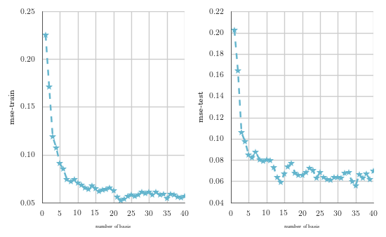
We show the mean square error train and test results for the MNIST handwritten digit classification problem as a function of the number of basis used in the least square residual classifier.
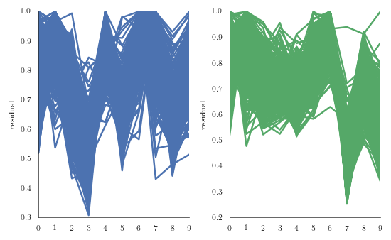
We now show the relative residual norm for all test digit 3 and all test digit 7 in terms of all 10 bases. We notice in the two figures, that most of the test digits 3 and 7 are best approximated in terms of their own basis.
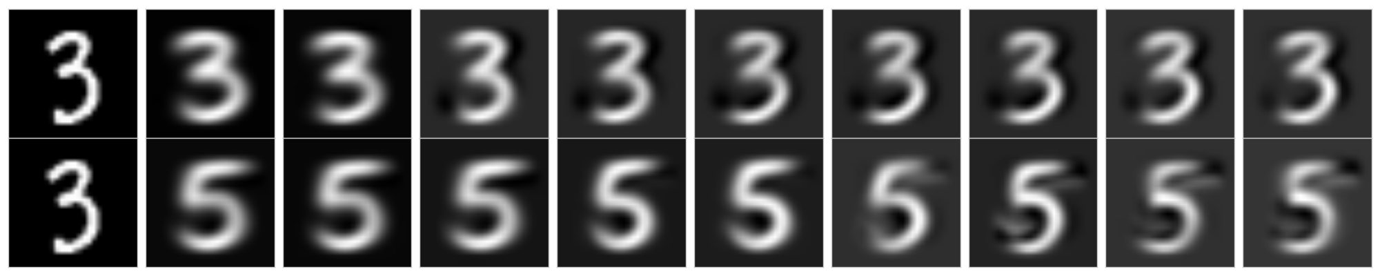
We show in the figure below the svd approximation of digit 3 using orthogonal basis with the different number of basis vectors 1 to 10. In the top panel, \(\mathbf{U}_3\) is used to compute the approximations of test digit 3 with increased basis from left to right and similarly bottom panel use \( \mathbf{U}_5\) to compute the svd approximations of 3.
We show now how the residual depends on the number of basis vectors. In the left panel, \(\mathbf{U}_3\) is used to compute the approximations of test digit 3 and similarly right panel use \(\mathbf{U}_5\) to compute the svd approximations of 3.
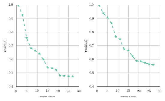
We see that the relative residual is considerably smaller in the basis \(\mathbf{U}_3\) than in the basis \(\mathbf{U}_5\)
Finally, though the least square residual classifier is quite fast in test phase and can be suitable for real time computations, they suffer to classify ugly digits.
The layout of this blog is inspired by Building Autoencoders in Keras
References
- Matrix Methods in Data Mining and Pattern Recognition
- Handwritten digit classification using higher order singular value decomposition
- Algorithms in data mining using matrix and tensor methods
- Analyses and Test of Handwritten Digit Recognition Algorithm